Agenda
📚 Parallel computing on CPUs & performance assessment, the metric
💻 Unit testing in Julia
🚧 Exercises:
CPU perf. codes for 2D diffusion and memcopy
Unit tests and testset implementation
How to assess the performance of numerical application?
Are you familiar the concept of wall-time?
What are the key ingredients to understand performance?
Performance limiters
Effective memory throughput metric
Parallel computing on CPUs
Shared memory parallelisation
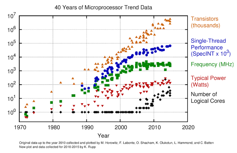
Recent processors (CPUs and GPUs) have multiple (or many) cores
Recent processors use their parallelism to hide latency (i.e. overlapping execution times (latencies) of individual operations with execution times of other operations)
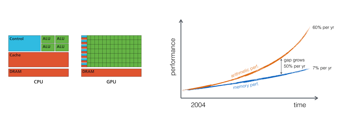
Multi-core CPUs and GPUs share similar challenges
Recall from lecture 1 (why we do it) ...
Use parallel computing (to address this):
The "memory wall" in ~ 2004
Single-core to multi-core devices
GPUs are massively parallel devices
SIMD machine (programmed using threads - SPMD) (more)
Further increases the FLOPS vs Bytes gap
Taking a look at a recent GPU and CPU:
Nvidia A100 GPU
Nvidia GH200 GPU
AMD EPYC "Rome" 7282 (16 cores) CPU
| Device | TFLOP/s (FP64) | Memory BW TB/s |
|---|---|---|
| Nvidia GH200 | 34 | 4 |
| Nvidia A100 | 9.7 | 1.55 |
| AMD EPYC 7282 | 0.7 | 0.085 |
Current GPUs (and CPUs) can do many more computations in a given amount of time than they can access numbers from main memory.
Quantify the imbalance:
(Theoretical peak performance values as specified by the vendors can be used).
Back to our hardware:
| Device | TFLOP/s (FP64) | Memory BW TB/s | Imbalance (FP64) |
|---|---|---|---|
| Nvidia GH200 | 34 | 4 | 34 / 4 × 8 = 68 |
| Nvidia A100 | 9.7 | 1.55 | 9.7 / 1.55 × 8 = 50 |
| AMD EPYC 7282 | 0.7 | 0.085 | 0.7 / 0.085 × 8 = 66 |
(here computed with double precision values)
Meaning: we can do ≥ 50 (GPU) and 66 (CPU) floating point operations per number accessed from main memory. Floating point operations are "for free" when we work in memory-bounded regimes
➡ Requires to re-think the numerical implementation and solution strategies
Most algorithms require only a few operations or FLOPS ...
... compared to the amount of numbers or bytes accessed from main memory.
First derivative example :
If we "naively" compare the "cost" of an isolated evaluation of a finite-difference first derivative, e.g., computing a flux :
which in the discrete form reads q[ix] = -D*(A[ix+1]-A[ix])/dx.
The cost of evaluating q[ix] = -D*(A[ix+1]-A[ix])/dx:
1 reads + 1 write => = 16 Bytes transferred
1 (fused) addition and division => 1 floating point operation
assuming:
, are scalars
and are arrays of Float64 (read from main memory)
GPUs and CPUs perform 50 - 60 floating-point operations per number accessed from main memory
First derivative evaluation requires to transfer 2 numbers per floating-point operations
The FLOPS metric is no longer the most adequate for reporting the application performance of many modern applications on modern hardware.
Need for a memory throughput-based performance evaluation metric: [GB/s]
➡ Evaluate the performance of iterative stencil-based solvers.
The effective memory access [GB]
Sum of:
twice the memory footprint of the unknown fields, , (fields that depend on their own history and that need to be updated every iteration)
known fields, , that do not change every iteration.
The effective memory access divided by the execution time per iteration, [sec], defines the effective memory throughput, [GB/s]:
The upper bound of is as measured, e.g., by McCalpin, 1995 for CPUs or a GPU analogue.
Defining the metric, we assume that:
we evaluate an iterative stencil-based solver,
the problem size is much larger than the cache sizes and
the usage of time blocking is not feasible or advantageous (reasonable for real-world applications).
As first task, we'll compute the for the 2D fluid pressure (diffusion) solver at the core of the porous convection algorithm from previous lecture.
👉 Download the script l6_Pf_diffusion_2D.jl to get started.
To-do list:
copy l6_Pf_diffusion_2D.jl, rename it to Pf_diffusion_2D_Teff.jl
add a timer
include the performance metric formulas
deactivate visualisation
💻 Let's get started
Use Base.time() to return the current timestamp
Define t_tic, the starting time, after 11 iterations steps to allow for "warm-up"
Record the exact number of iterations (introduce e.g. niter)
Compute the elapsed time t_toc at the end of the time loop and report:
t_toc = Base.time() - t_tic
A_eff = (3*2)/1e9*nx*ny*sizeof(Float64)  # Effective main memory access per iteration [GB]
t_it  = t_toc/niter                      # Execution time per iteration [s]
T_eff = A_eff/t_it                       # Effective memory throughput [GB/s]
Report t_toc, T_eff and niter at the end of the code, formatting output using @printf() macro.
Round T_eff to the 3rd significant digit.
@printf("Time = %1.3f sec, T_eff = %1.2f GB/s (niter = %d)\n", t_toc, round(T_eff, sigdigits=3), niter)Use keyword arguments ("kwargs") to allow for default behaviour
Define a do_check flag set to false
function Pf_diffusion_2D(;do_check=false)
    if do_check && (iter%ncheck == 0)
    ...
    end
    return
end
So far so good, we have now a timer.
Let's also boost resolution to nx = ny = 511 and set maxiter = max(nx,ny) to have the code running ~1 sec.
In the next part, we'll work on a multi-threading implementation.
Towards implementing shared memory parallelisation using multi-threading capabilities of modern multi-core CPUs.
We'll work it out in 3 steps:
Precomputing scalars, removing divisions (and non-necessary arrays)
Back to loops I
Back to loops II - compute functions (future "kernels")
Precomputing scalars, removing divisions and casual arrays
Let's duplicate Pf_diffusion_2D_Teff.jl and rename it as Pf_diffusion_2D_perf.jl.
First, replace k_ηf/dx and k_ηf/dy in the flux calculations by inverse multiplications, such that
k_ηf_dx, k_ηf_dy = k_ηf/dx, k_ηf/dyThen, replace divisions ./(1.0 + θ_dτ) by inverse multiplications *_1_θ_dτ such that
_1_θ_dτ = 1.0./(1.0 + θ_dτ)Then, replace ./dx and ./dy in the Pf update by inverse multiplications *_dx, *_dy where
_dx, _dy = 1.0/dx, 1.0/dyFinally, also apply the same treatment to ./β_dτ
Back to loops I
As first, duplicate Pf_diffusion_2D_perf.jl and rename it as Pf_diffusion_2D_perf_loop.jl.
The goal is now to write out the diffusion physics in a loop fashion over and dimensions.
Implement a nested loop, taking car of bounds and staggering.
for iy=1:ny
    for ix=1:nx-1
        qDx[ix+1,iy] -= (qDx[ix+1,iy] + k_ηf_dx*(Pf[ix+1,iy]-Pf[ix,iy]))*_1_θ_dτ
    end
end
for iy=1:ny-1
    for ix=1:nx
        qDy[ix,iy+1] -= (qDy[ix,iy+1] + k_ηf_dy*(Pf[ix,iy+1]-Pf[ix,iy]))*_1_θ_dτ
    end
end
for iy=1:ny
    for ix=1:nx
        Pf[ix,iy]  -= ((qDx[ix+1,iy]-qDx[ix,iy])*_dx + (qDy[ix,iy+1]-qDy[ix,iy])*_dy)*_β_dτ
    end
end
We could now use macros to make the code nicer and clearer. Macro expression will be replaced during pre-processing (prior to compilation). Also, macro can take arguments by appending $ in their definition.
Let's use macros to replace the derivative implementations
macro d_xa(A)  esc(:( $A[ix+1,iy]-$A[ix,iy] )) end
macro d_ya(A)  esc(:( $A[ix,iy+1]-$A[ix,iy] )) end
And update the code within the iteration loop:
for iy=1:ny
    for ix=1:nx-1
        qDx[ix+1,iy] -= (qDx[ix+1,iy] + k_ηf_dx*@d_xa(Pf))*_1_θ_dτ
    end
end
for iy=1:ny-1
    for ix=1:nx
        qDy[ix,iy+1] -= (qDy[ix,iy+1] + k_ηf_dy*@d_ya(Pf))*_1_θ_dτ
    end
end
for iy=1:ny
    for ix=1:nx
        Pf[ix,iy]  -= (@d_xa(qDx)*_dx + @d_ya(qDy)*_dy)*_β_dτ
    end
end
Performance is already quite better with the loop version 🚀.
Reasons are that diff() are allocating and that Julia is overall well optimised for executing loops.
Let's now implement the final step.
Back to loops II
Duplicate Pf_diffusion_2D_perf_loop.jl and rename it as Pf_diffusion_2D_perf_loop_fun.jl.
In this last step, the goal is to define compute functions to hold the physics calculations, and to call those within the time loop.
Create a compute_flux!() and compute_Pf!() functions that take input and output arrays and needed scalars as argument and return nothing.
function compute_flux!(qDx,qDy,Pf,k_ηf_dx,k_ηf_dy,_1_θ_dτ)
    nx,ny=size(Pf)
    for iy=1:ny,
        for ix=1:nx-1
            qDx[ix+1,iy] -= (qDx[ix+1,iy] + k_ηf_dx*@d_xa(Pf))*_1_θ_dτ
        end
    end
    for iy=1:ny-1
        for ix=1:nx
            qDy[ix,iy+1] -= (qDy[ix,iy+1] + k_ηf_dy*@d_ya(Pf))*_1_θ_dτ
        end
    end
    return nothing
end

function update_Pf!(Pf,qDx,qDy,_dx,_dy,_β_dτ)
    nx,ny=size(Pf)
    for iy=1:ny
        for ix=1:nx
            Pf[ix,iy]  -= (@d_xa(qDx)*_dx + @d_ya(qDy)*_dy)*_β_dτ
        end
    end
    return nothing
end! in their name, a Julia convention.The compute_flux!() and compute_Pf!() functions can then be called within the time loop.
This last implementation executes a bit faster as previous one, as functions allow Julia to further optimise during just-ahead-of-time compilation.
@inbounds in front of the compute statement, or running the scripts (or launching Julia) with the --check-bounds=no option.Various timing and benchmarking tools are available in Julia's ecosystem to track performance issues. Julia's Base exposes the @time macro which returns timing and allocation estimation. BenchmarkTools.jl package provides finer grained timing and benchmarking tooling, namely the @btime, @belapsed and @benchmark macros, among others.
Let's evaluate the performance of our code using BenchmarkTools. We will need to wrap the two compute kernels into a compute!() function in order to be able to call that one using @belapsed. Query ? @belapsed in Julia's REPL to know more.
The compute!() function:
function compute!(Pf,qDx,qDy,k_ηf_dx,k_ηf_dy,_1_θ_dτ,_dx,_dy,_β_dτ)
    compute_flux!(qDx,qDy,Pf,k_ηf_dx,k_ηf_dy,_1_θ_dτ)
    update_Pf!(Pf,qDx,qDy,_dx,_dy,_β_dτ)
    return nothing
end
can then be called using @belapsed to return elapsed time for a single iteration, letting BenchmarkTools taking car about sampling
t_toc = @belapsed compute!($Pf,$qDx,$qDy,$k_ηf_dx,$k_ηf_dy,$_1_θ_dτ,$_dx,$_dy,$_β_dτ)
niter = 1$ in front.Julia ships with it's Base feature the possibility to enable multi-threading.
The only 2 modifications needed to enable it in our code are:
Place Threads.@threads in front of the outer loop definition
Export the desired amount of threads, e.g., export JULIA_NUM_THREADS=4, to be activate prior to launching Julia (or executing the script from the shell). You can also launch Julia with -t option setting the desired numbers of threads. Setting -t auto will most likely automatically use as many hardware threads as available on a machine.
The number of threads can be queried within a Julia session as following: Threads.nthreads()
Julia's ecosystem offers various approaches to try supporting SIMD operations.
Using LoopVectorization.jl, it is possible to combine multi-threading with advanced vector extensions (AVX) optimisations, leveraging extensions to the x86 instruction set architecture.
Julia base also exposes @simd macro that would possibly enable the compiler to take extra liberties to allow loop re-ordering.
To enable LoopVectorization:
Add using LoopVectorization at the top of the script
Replace Threads.@threads by @tturbo
To try making use of SIMD, decorate the for loop with @simd for.
We discussed main performance limiters
We implemented the effective memory throughput metric
We optimised the Julia 2D diffusion code (multi-threading and AVX)
Test moduleBasic unit tests in Julia
Provides simple unit testing functionality
A way to assess if code is correct by checking that results are as expected
Helpful to ensure the code still works after changes
Can be used when developing
Should be used in package for continous integration (aka CI; when tests are run on GitHub automatically on a push)
Simple unit testing can be performed with the @test and @test_throws macros:
using Test

@test 1==1

@test_throws MethodError 1+"a" ## the expected error must be provided too
Or another example
@test [1, 2] + [2, 1] == [3, 3]Testing an expression which is a call using infix syntax such as approximate comparisons (\approx + tab)
@test π ≈ 3.14 atol=0.01For example, suppose we want to check our new function square(x) works as expected:
square(x) = x^2If the condition is true, a Pass is returned:
@test square(5) == 25If the condition is false, then a Fail is returned and an exception is thrown:
@test square(5) == 20Test Failed at none:1
Expression: square(5) == 20
Evaluated: 25 == 20
Test.FallbackTestSetException("There was an error during testing")The @testset macro can be used to group tests into sets.
All the tests in a test set will be run, and at the end of the test set a summary will be printed.
If any of the tests failed, or could not be evaluated due to an error, the test set will then throw a TestSetException.
@testset "trigonometric identities" begin
    θ = 2/3*π
    @test sin(-θ) ≈ -sin(θ)
    @test cos(-θ) ≈ cos(θ)
    @test sin(2θ) ≈ 2*sin(θ)*cos(θ)
    @test cos(2θ) ≈ cos(θ)^2 - sin(θ)^2
end;
Let's try it with our square() function
square(x) = x^2

@testset "Square Tests" begin
    @test square(5) == 25
    @test square("a") == "aa"
    @test square("bb") == "bbbb"
end;
If we now introduce a bug
square(x) = x^2

@testset "Square Tests" begin
    @test square(5) == 25
    @test square("a") == "aa"
    @test square("bb") == "bbbb"
    @test square(5) == 20
end;
Square Tests: Test Failed at none:6
Expression: square(5) == 20
Evaluated: 25 == 20
Stacktrace:
[...]
Test Summary: | Pass Fail Total
Square Tests | 3 1 4
Some tests did not pass: 3 passed, 1 failed, 0 errored, 0 broken.Then then the reporting tells us a test failed.
The simplest is to just put the tests in your script, along the tested function. Then the tests run every time the script is executed.
However, for bigger pieces of software, such as packages, this becomes unwieldly and also undesired (as we don't want tests to run all the time). Then tests are put into test/runtests.jl. If they are there they will be run when called from package mode or from automated test (CI).
Example for the package Literate.jl (we use that to generate the website):
julia> using Pkg

julia> Pkg.test("Literate")
     Testing Literate
   ...
     Testing Running tests...
Test Summary:  | Pass  Total  Time
Literate.parse |  533    533  0.8s
Test Summary:   | Pass  Broken  Total  Time
Literate.script |   36       1     37  2.1s
Test Summary:     | Pass  Broken  Total  Time
Literate.markdown |   82       2     84  4.3s
Test Summary:     | Pass  Broken  Total  Time
Literate.notebook |   86       1     87  5.2s
Test Summary: | Pass  Total  Time
Configuration |    7      7  0.3s
Testing Literate tests passedThe Test module provides simple unit testing functionality.
Tests can be grouped into sets using @testset.
We'll later see how tests can be used in CI.
👉 See Logistics for submission details.
The goal of this exercise is to:
Finalise the script discussed in class
In this first exercise, you will terminate the performance oriented implementation of the 2D fluid pressure (diffusion) solver script from lecture 6.
👉 If needed, download the l6_Pf_diffusion_2D.jl to get you started.
Create a new folder in your GitHub repository for this week's (lecture 6) exercises. In there, create a new subfolder Pf_diffusion_2D where you will add following script:
Pf_diffusion_2D_Teff.jl: T_eff implementation
Pf_diffusion_2D_perf.jl: scalar precomputations and removing disabling ncheck
Pf_diffusion_2D_loop_fun.jl: physics computations in compute!() function, derivatives done with macros, and multi-threading
👉 See Logistics for submission details.
The goal of this exercise is to:
Create a script to assess , using memory-copy
Assess of your CPU
Perform a strong-scaling test: assess for the fluid pressure diffusion 2D solver as function of number of grid points and implementation
For this exercise, you will write a code to assess the peak memory throughput of your CPU and run a strong scaling benchmark using the fluid pressure diffusion 2D solver and report performance.
In the Pf_diffusion_2D folder, create a new script named memcopy.jl. You can use as starting point the diffusion_2D_loop_fun.jl script from lecture 6 (or exercise 1).
Rename the "main" function memcopy()
Modify the script to only keep following in the initialisation:
# Numerics
nx, ny  = 512, 512
nt      = 2e4
# array initialisation
C       = rand(Float64, nx, ny)
C2      = copy(C)
A       = copy(C)
Implement 2 compute functions to perform the following operation C2 = C + A, replacing the previous calculations:
create an "array programming"-based function called compute_ap!() that includes a broadcasted version of the memory copy operation;
create a second "kernel programming"-based function called compute_kp!() that uses a loop-based implementation with multi-threading.
Update the A_eff formula accordingly.
Implement a switch to monitor performance using either a manual approach or BenchmarkTools and pass the bench value as kwarg to the memcopy() main function including a default:
if bench == :loop
    # iteration loop
    t_tic = 0.0
    for iter=1:nt
      ...
    end
    t_toc = Base.time() - t_tic
elseif bench == :btool
    t_toc = @belapsed ...
end
Then, create a README.md file in the Pf_diffusion_2D folder to report the results for each of the following tasks (including a .png of the figure when instructed)
 to insert a .png figure in the README.md.Report on a figure of your memcopy.jl code as function of number of grid points nx × ny for the array and kernel programming approaches, respectively, using the BenchmarkTools implementation. Vary nxand ny such that
nx = ny = 16 * 2 .^ (1:8)( of your memcopy.jl code represents , the peak memory throughput you can achieve on your CPU for a given implementation.)
On the same figure, report the best value of memcopy obtained using the manual loop-based approach (manual timer) to assess .
nt accordingly (you could also, e.g., make nt function of nx, ny). Ensure also to implement "warm-up" iterations.Add the above figure in a new section of the Pf_diffusion_2D/README.md, and provide a minimal description of 1) the performed test, and 2) a short description of the result. Figure out the vendor-announced peak memory bandwidth for your CPU, add it to the figure and use it to discuss your results.
Repeat the strong scaling benchmark you just realised in Task 2 using the various fluid pressure diffusion 2D codes (Pf_diffusion_2D_Teff.jl; Pf_diffusion_2D_perf.jl; Pf_diffusion_2D_loop_fun.jl - with/without Threads.@threads for the latter).
Report on a figure of the 4 diffusion solvers' implementations as function of number of grid points nx × ny. Vary nxand ny such that nx = ny = 16 * 2 .^ (1:8). Use the BenchmarlTools-based evaluation approach.
On the same figure, report also the best memory copy value (as, e.g, dashed lines) and vendor announced values (if available - optional).
Add this second figure in a new section of the Pf_diffusion_2D/README.md, and provide a minimal description of 1) the performed test, and 2) a short description of the result.
👉 See Logistics for submission details.
The goal of this exercise is to:
Implement basic unit tests for the diffusion and acoustic 2D scripts
Group the tests in a test-set
For this exercise, you will implement a test set of basic unit tests using Julia's built-in testing infrastructure to verify the implementation of the diffusion and acoustic 2D solvers.
In the Pf_diffusion_2D folder, duplicate the Pf_diffusion_2D_perf_loop_fun.jl script and rename it Pf_diffusion_2D_test.jl.
Implement a test set using @testset and @test macros from Test.jl in order to test Pf[xtest, ytest] and assess that the values returned are approximatively equal to the following ones for the given values of nx = ny. Make sure to set do_check = false i.e. to ensure the code to run 500 iterations.
xtest = [5, Int(cld(0.6*lx, dx)), nx-10]
ytest = Int(cld(0.5*ly, dy))
for
nx = ny = 16 * 2 .^ (2:5) .- 1
maxiter = 500
should match
nx, ny | Pf[xtest, ytest] |
|---|---|
63 | [0.00785398056115133 0.007853980637555755 0.007853978592411982] |
127 | [0.00787296974549236 0.007849556884184108 0.007847181374079883] |
255 | [0.00740912103848251 0.009143711648167267 0.007419533048751209] |
511 | [0.00566813765849919 0.004348785338575644 0.005618691590498087] |
Report the output of the test set as code block in a new section of the README.md in the Pf_diffusion_2D folder.
README.md (more).