Lecture 2

Agenda
📚 PDEs and physical processes – diffusion, wave propagation, advection
💻 Get started on GitHub
🚧 Exercises:

• Basic code structure & vectorisation

• Combine physical processes

• First steps on Git

---

Content

👉 get started with exercises

---

PDEs and physical processes

diffusion, wave propagation, advection

The goal of this lecture 2 is to familiarise (or refresh) with

• Partial differential equations - PDEs (e.g. diffusion and advection equations)

• Finite-difference discretisation

• Explicit solutions

• Nonlinear processes

• Multi-process (physics) coupling

A partial differential equation (PDE) is an equation which imposes relations between the various partial derivatives of a multivariable function. Wikipedia

Parabolic PDEs - diffusion

The diffusion equation was introduced by Fourier in 1822 to understand heat distribution (heat equation) in various materials.

Diffusive processes were also employed by Fick in 1855 with application to chemical and particle diffusion (Fick's law).

The diffusion equation is often reported as a second order parabolic PDE, here for a multivariable function $C(x,t)$ showing derivatives in both temporal $∂t$ and spatial $∂x$ dimensions (here for the 1D case)

$$\frac{∂C}{∂t} = D\frac{∂^2 C}{∂ x^2}~,$$

where $D$ is the diffusion coefficient.

A more general description combines a diffusive flux:

$$q = -D\frac{∂C}{∂x}~,$$

and a conservation or flux balance equation:

$$\frac{∂C}{∂t} = -\frac{∂q}{∂x}~.$$

To discretise the diffusion equation, we will keep the explicit forward Euler method as temporal discretisation and use finite-differences for the spatial discretisation.

Finite-differences discretisation on regular staggered grid allows for concise and performance oriented algorithms, because only neighbouring cell access is needed to evaluate gradient and data alignment is natively pretty optimal.

A long story short, we will approximate the gradient of a quantity $C$ (e.g., concentration) over a distance $∂x$, a first derivative $\frac{∂C}{∂x}$, we will perform following discrete operation

$$\frac{C_{x+dx} - C_{x}}{dx}~,$$

where $dx$ is the discrete size of the cell.

The same reasoning also applies to the flux balance equation.

We can use Julia's diff() operator to apply the $C_{x+dx} - C_{x}$,

C[ix+1] - C[ix]

in a vectorised fashion to our entire C vector as

diff(C)

So, we are ready to solve the 1D diffusion equation.

We introduce the physical parameters that are relevant for the considered problem, i.e., the domain length lx and the diffusion coefficient dc:

# physics
lx   = 20.0
dc   = 1.0

Then we declare numerical parameters: the number of grid cells used to discretize the computational domain nx, and the frequency of updating the visualisation nvis:

# numerics
nx   = 200
nvis = 5

We introduce additional numerical parameters: the grid spacing dx and the coordinates of cell centers xc:

# derived numerics
dx   = lx/nx
xc   = LinRange(dx/2,lx-dx/2,nx)

In the # array initialisation section, we need to initialise one array to store the concentration field C, and the diffusive flux in the x direction qx:

# array initialisation
C    = @. 0.5cos(9π*xc/lx)+0.5; C_i = copy(C)
qx   = zeros(Float64, nx-1)

Wait... why it wouldn't work?

👉 Your turn. Let's implement our first diffusion solver trying to think about how to solve the staggering issue.

The initialisation steps of the diffusion code should contain

# physics
lx   = 20.0
dc   = 1.0
# numerics
nx   = 200
nvis = 5
# derived numerics
dx   = lx/nx
dt   = dx^2/dc/2
nt   = nx^2 ÷ 100
xc   = LinRange(dx/2,lx-dx/2,nx)
# array initialisation
C    = @. 0.5cos(9π*xc/lx)+0.5; C_i = copy(C)
qx   = zeros(Float64, nx-1)

Followed by the 3 physics computations (lines) in the time loop

# time loop
for it = 1:nt
    qx          .= .-dc.*diff(C )./dx
    C[2:end-1] .-=   dt.*diff(qx)./dx
    # visualisation
end

One can examine the size of the various vectors ...

# check sizes and staggering
@show size(qx)
@show size(C)
@show size(C[2:end-1])

... and visualise it

using Plots
plot( xc               , C , label="Concentration"        , linewidth=:1.0, markershape=:circle, markersize=5, framestyle=:box)
plot!(xc[1:end-1].+dx/2, qx, label="flux of concentration", linewidth=:1.0, markershape=:circle, markersize=5, framestyle=:box)

Note: plotting and visualisation is slow. A convenient workaround is to only visualise or render the figure every nvis iteration within the time loop

@gif for it = 1:nt
    # plot(...)
end every nvis

👉 Download the l2_diffusion_1D.jl script

Hyperbolic PDEs - acoustic wave propagation

The wave equation

... is a second-order partial differential equation.

The wave equation is a second-order linear partial differential equation for the description of waves—as they occur in classical physics—such as mechanical waves (e.g. water waves, sound waves and seismic waves) or light waves. Wikipedia

The hyperbolic equation reads

$$\frac{∂^2P}{∂t^2} = c^2 ∇^2 P~,$$

where

• $P$ is pressure (or, displacement, or another scalar quantity...)

• $c$ a real constant (speed of sound, stiffness, ...)

The wave equation can be elegantly derived, e.g., from Hooke's law and second law of Newton considering masses interconnected with springs.

$$F_\mathrm{Newton}~~=~~F_\mathrm{Hook}~,$$ $$m⋅a(t)~~=~~k x_+ - k x_-~,$$

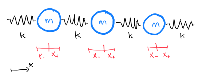
where $m$ is the mass, $k$ de spring stiffness, and $x_+$, $x_-$ the oscillations of the masses (small distances).

The acceleration $a(t)$ can be substituted by the second derivative of displacement $u$ as function of time $t$, $∂^2u/∂t^2$, while balancing $x_+ - x_-$ and taking the limit leads to $∂^2u/∂x^2$.

Back to the wave equation

The objective is to implement the wave equation in 1D (spatial discretisation) using an explicit time integration (forward Euler) as for the diffusion physics.

Our first task will be to modify the diffusion equation...

... in order to obtain and implement the acoustic wave equation:

From diffusion to acoustic wave propagation

We won't implement first the hyperbolic equation as introduced, but rather start from a first order system, similar to the one that we used to implement the diffusion equation.

To this end, we can rewrite the second order wave equation

$$\frac{∂^2 P}{∂t^2} = c^2 ∇^2 P~,$$

as two first order equations

$$\frac{∂V_x}{∂t} = -\frac{1}{ρ}~\frac{∂P}{∂x}~,$$ $$\frac{∂P}{∂t} = -\frac{1}{\beta}~\frac{∂V_x}{∂x}~.$$

Let's get started.

👉 Download the l2_diffusion_1D.jl script to get you started

We can start modifying the diffusion code's, adding ρ and β in # physics section, and taking a Gaussian (centred in lx/2) as initial condition for the pressure Pr

# physics
lx   = 20.0
ρ,β  = 1.0,1.0

# array initialisation
Pr  =  @. exp(-(xc - lx/4)^2)

Then, the diffusion physics:

qx          .= .-dc.*diff(C )./dx
C[2:end-1] .-=   dt.*diff(qx)./dx

Should be modified to account for pressure Pr instead of concentration C, the velocity update (Vx) added, and the coefficients modified:

Vx          .-= dt./ρ.*diff(Pr)./dx
Pr[2:end-1] .-= dt./β.*diff(Vx)./dx

👉 Download the acoustic_1D.jl script for comparison.

Compare the equations

Comparing diffusive and wave physics, we can summarise following:

Diffusion	Wave propagation
$q = -D\frac{\partial C}{\partial x}$	$\frac{\partial V_x}{\partial t} = -\frac{1}{\rho}\frac{\partial P}{\partial x}$
$\frac{\partial C}{\partial t} = -\frac{\partial q}{\partial x}$	$\frac{\partial P}{\partial t} = -\frac{1}{\beta}\frac{\partial V_x}{\partial x}$

First-order PDEs - advection

Advection is a partial differential equation that governs the motion of a conserved scalar field as it is advected by a known velocity vector field. Wikipedia

We will here briefly discuss advection of a quantity $C$ by a constant velocity $v_x$ in the one-dimensional x-direction.

$$\frac{∂C}{∂t} = -\frac{∂(v_x~C)}{∂x} ~.$$

In case the flow is incompressible ($\nabla\cdot v = 0$ - here $\nabla\cdot v = \frac{∂v_x}{∂x}$), the advection equation can be rewritten as

$$\frac{∂C}{∂t} = -v_x \frac{∂C}{∂x} ~.$$

Let's implement the advection equation, following the same code structure as for the diffusion and the acoustic wave propagation.

# physics
lx   = 20.0
vx   = 1.0

The only change in the # derived numerics section is the numerical time step definition to comply with the CFL condition for explicit time integration.

# derived numerics
dt   = dx/abs(vx)

In the # array initialisation section, initialise the quantity C as a Gaussian profile of amplitude 1, standard deviation 1, with centre located at $c = 0.4 l_x$.

C = @. exp(-(xc - lx/4)^2)

Update C as following:

C .-= dt.*vx.*diff(C)./dx # doesn't work

This doesn't work because of the mismatching array sizes.

There are at least three (naive) ways to solve the problem: update C[1:end-1], C[2:end], or one could even update C[2:end-1] with the spatial average of the rate of change dt.*vx.*diff(C)./dx.

👉 Your turn. Try it out yourself and motivate your best choice.

Here we go, an upwind approach is needed to implement a stable advection algorithm

C[2:end]   .-= dt.*vx.*diff(C)./dx # if vx>0
C[1:end-1] .-= dt.*vx.*diff(C)./dx # if vx<0

👉 Download the advection_1D.jl script

Nonlinear equations

Previously, we considered only linear equations, which means that the functions being differentiated depend only linearly on the unknown variables. A lot of important physical processes are essentially nonlinear, and could be only described by nonlinear PDEs.

A model of nonlinear parabolic PDE frequently arising in physics features nonlinearity of a power-law type:

$$\frac{\partial C}{\partial t} - D\frac{\partial^2 C^n}{\partial x^2} = 0$$

where $n$ is a power-law exponent (here $n=4$).

Such equations describe the deformation of shallow currents of fluids with high viscosity such as ice or lava under their own weight, or evolution of pressure in elastic porous media.

A model of nonlinear advection equation is often referred to as inviscid Burgers' equation:

$$\frac{\partial C}{\partial t} + v_x \frac{\partial C^n}{\partial x} = 0$$

where $n$ is often assumed to be equal to 2. This equation describes the formation of shock waves.

First step towards solving the elliptic problem

We have considered numerical solutions to the hyperbolic and parabolic PDEs.

In both cases we used the explicit time integration

The elliptic PDE is different:

$$\frac{\partial^2 C}{\partial x^2} = 0$$

It doesn't depend on time! How do we solve it numerically then?

Solution to the elliptic PDE

... is the steady state limit of the time-dependent diffusion problem described by the parabolic PDE:

$$\frac{\partial^2 C}{\partial x^2} - \frac{\partial C}{\partial t} = 0$$

when $t\rightarrow\infty$, and we know how to solve parabolic PDEs.

Let's try to increase the number of time steps nt in our diffusion code to see whether the solution would converge, and decrease the frequency of plotting:

nt   = nx^2 ÷ 5
nvis = 50

and see the results:

We approach the steady-state, but the number of time steps required to converge to a solution is proportional to nx^2.

• For simulations in 1D and low resolutions in 2D the quadratic scaling is acceptable.

• For high-resolution 2D and 3D the nx^2 factor becomes prohibitively expensive!

We'll handle this problem in the next lecture, stay tuned! 🚀

Wrapping-up

• We implemented and solved PDEs for diffusion, wave propagation, and advection processes in 1D

• We used conservative staggered grid finite-differences, explicit forward Euler time stepping and upwind scheme for advection.

Note that this is far from being the only way to tackle numerical solutions to these PDEs. In this course, we will stick to those concepts as they will allow for efficient GPU (parallel) implementations.

⤴ back to Content

A brief intro to Git

Git is a version control software, useful to

• keep track of your progress on code (and other files)

• to collaborate on code

• to distribute code, to onself (on other computers) and others

Previous experience

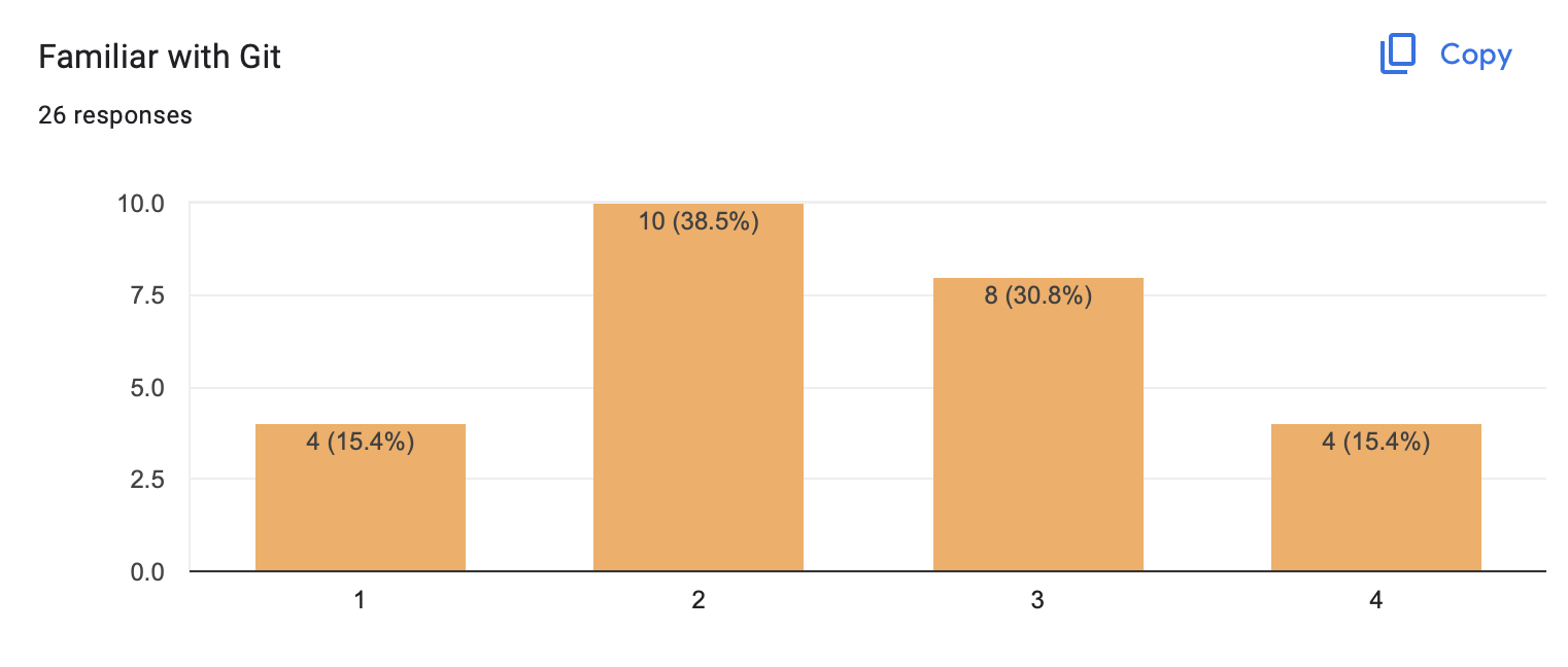
You are familiar with git already:

Questions:

• how often do you use git?

• who has git installed on their laptop?

• do you use: commit, push, pull, clone?

• do you use: branch, merge, rebase?

• GitHub/GitLab etc?

A brief git demo session

Please follow along!

If you don't have git installed, head to JupyterHub (within Moodle) and open a terminal. (And do install it on your computer!)

• git setup:

git config --global user.name "Your Name"
git config --global user.email "youremail@yourdomain.com"

• make a repo (init)

• add some files (add, commit)

• do some changes (commit some more)

• make a feature branch (branch, diff, difftool)

• merge branch (merge)

• tag (tag)

Further reading

There are (too) many resources on the web...

• book: https://git-scm.com/book/en/v2

• videos: https://git-scm.com/doc

• cheat sheet (click on boxes) https://www.ndpsoftware.com/git-cheatsheet.html#loc=workspace;

• get out of a git mess: http://justinhileman.info/article/git-pretty/git-pretty.png

Other tools for git

There is plenty of software to interact with git, graphical, command line, VSCode, etc. Feel free to use those.

But we will only be able to help you with vanilla, command-line git.

Getting started on GitHub (similar on GitLab, or elsewhere)

GitHub and GitLab are social coding websites

• they host code

• they facilitate for developers to interact

• they provide infrastructure for software testing, deployment, etc

Question: who has a GitHub account?

Let's make one (because most of Julia development happens on GitHub)

https://github.com/ -> "Sign up"

GitHub setup

Make such that you can push and pull without entering a password

• local: tell git to store credentials: git config --global credential.helper cache (this may not be needed on all operating systems, potentially a built-in password/credential manager will do this automatically)

• github.com:

  • "Settings" -> "Developer settings" -> "Personal access tokens" -> "Generate new token"

    • Give the token a description/name and select the scope of the token

    • I selected "repo only" to facilitate pull, push, clone, and commit actions

  • -> "Generate token" and copy it (keep that website open for now)

Let's get our repo onto GitHub

• create a repository on github.com: click the "+"

• local: follow setup given on website

• local: git push

  • here enter your username + the token generated before

Work with other people: pull request (PR)

When you contribute new code to a repo (in particular a repo which other people work on too), the new code is submitted via a "pull request". This code is then in a separate branch. A pull request then makes a web-interface where one can review the changes, request amendments and finally merge the code.

In a repo with write permission, the use following work-flow:

• make a branch and switch to it: git switch -c some-branch-name

• make changes, add files, etc. and commit to the branch. You can have several commits on the branch.

• push the branch to Github

• on the Github web-page a bar with a "open pull request" should show: click it

• if you got more changes, just commit and push them to that branch

• when happy merge the PR

This work-flow you will use to submit homework for the course.

Work with other peoples code: fork

For repos without write access, to contribute do:

• fork a repository on github.com (top right)

• make a branch on that fork and work on it

• push that to github and open a PR with respect to that fork

• (not needed in this lecture course)

Git: questions?

⤴ back to Content

Exercises - lecture 2

Exercise 1 - Advection-Diffusion

👉 Download the notebook to get started with this exercise!

The goal of this exercise is to couple physical processes implementing:

• 1D advection-diffusion

• Non-dimensional numbers

The goal of this exercise is to combine advection and diffusion processes acting on the concentration of a quantity $C$.

From what you learned in class, write an advection-diffusion code having following physical input parameters:

# Physics
lx   = 20.0  # domain length
dc   = 0.1   # diffusion coefficient
vx   = 1.0   # advection velocity
ttot = 20.0  # total simulation time

Discretise your domain in 200 finite-difference cells such that the first cell centre is located at dx/2 and the last cell centre at lx-dx/2. Use following explicit time step limiters:

dta  = dx/abs(vx)
dtd  = dx^2/dc/2
dt   = min(dtd, dta)

As initial condition, define a Gaussian profile of concentration C of amplitude and standard deviation equal to 1, located at lx/4.

In the time-loop, add a condition that would change de direction of the velocity vx at time ttot/2.

Set Dirichlet boundary conditions on the concentration for the diffusion process such that C=0 at the boundaries. This can be implicitly achieved by updating only the inner points of C with the divergence of the diffusive flux (i.e. C[2:end-1]). For the advection part, implement upwind scheme making sure to treat cases for both positive and negative velocities vx.

Question 1

Report the initial and final distribution of concentration on a figure with axis-label, title, and plotted line labels. Also, report on the figure (as text in one label of your choice) the maximal final concentration value and its x location.

Question 2

Repeat the exercise but introduce the non-dimensional Péclet number $Pe = lx~vx/dc$ as physical quantity defining the diffusion coefficient dc as a # Derived physics quantity. Confirm the if $Pe >> 100$ the diffusion happens in a much longer time compared to the advection, and the opposite for $Pe << 100$.

⤴ back to Content

---

Exercise 2 - Reaction-Diffusion

👉 Download the notebook to get started with this exercise!

The goal of this exercise is to couple physical processes implementing:

• 1D reaction-diffusion

• Non-dimensional numbers

The goal of this exercise is to combine reaction and diffusion processes acting on the concentration of a quantity $C$. The reaction equation is an ODE, as the evolution of the quantity $C$ does not depend on the neighbouring values (or spatial gradients). Consider the following reaction ODE

$$\frac{∂C}{∂t} = -\frac{(C-C_\mathrm{eq})}{ξ}~,$$

where $C_\mathrm{eq}$ is the equilibrium concentration and $ξ$ the reaction rate.

From what you learned in class, write an reaction-diffusion code having following physical input parameters:

# Physics
lx   = 20.0  # domain length
dc   = 0.1   # diffusion coefficient
ξ    = 10.0  # reaction rate
Ceq  = 0.4   # equilibrium concentration
ttot = 20.0  # total simulation time

Discretise your domain in 200 finite-difference cells such that the first cell centre is located at dx/2 and the last cell centre at lx-dx/2. Use following explicit time step limiters:

dt   = dx^2/dc/2

As initial condition, define a Gaussian profile of concentration C of amplitude and standard deviation equal to 1, located at lx/4.

Update all entries of the array for the reaction process (ODE) but only inner points for the diffusion process (PDE), thus leading to the fact that boundary points will only be affected by reaction and not diffusion.

Question 1

Report the initial and final distribution of concentration on a figure with axis-label, title, and plotted line labels. Also, report on the figure (as text in one label of your choice) the maximal final concentration value and its $x$ location.

Question 2

Repeat the exercise but introduce the non-dimensional Damköhler number $Da = lx^2/dc/ξ$ as physical quantity defining the diffusion coefficient dc as a # Derived physics quantity. Confirm the if $Da < 0.1$ most of the mass diffuses away from $C_{eq}$, and the opposite holds for $Da > 1000$.

⤴ back to Content

---

Exercise 3 - Nonlinear problems

👉 Download the notebook to get started with this exercise!

The goal of this exercise is to consolidate:

• Nonlinear processes

• Advection and diffusion

The goal of this exercise is to program two short 1D codes to experiment with nonlinear processes, namely nonlinear diffusion and advection in order to reproduce the animations displayed in the nonlinear equations section of the lecture 2.

Task 1

Referring to the nonlinear equations section in lecture 2, implement the nonlinear power-law type parabolic PDE in 1D:

$$\frac{\partial C}{\partial t} - D\frac{\partial^2 C^n}{\partial x^2} = 0$$

Use one of your previous scripts or the l2_diffusion_1D.jl to get you started. Use the following parameters:

# physics
lx   = 20.0
dc   = 1.0
n    = 4
# numerics
nx   = 200
nvis = 50
# derived numerics
dx   = lx/nx
dt   = dx^2/dc/10
nt   = nx^2 ÷ 5
xc   = LinRange(dx/2,lx-dx/2,nx)

and initialising your quantity to diffuse as 0.5cos(9π*xc/lx)+0.5.

Make sure your code reproduces the animation from the course (alternatively, provide 5 snapshot-plots of the simulation evolution).

Task 2

Referring to the nonlinear equations section in lecture 2, implement the nonlinear advection inviscid Burgers' equation in 1D:

$$\frac{\partial C}{\partial t} + v_x \frac{\partial C^n}{\partial x} = 0$$

Use one of your previous scripts or the diffusion_1D.jl to get you started. Use the following parameters:

# physics
lx   = 20.0
vx   = 1.0
n    = 2
# numerics
nx   = 1000
nvis = 15
# derived numerics
dx   = lx/nx
dt   = dx/abs(vx)/2
nt   = 2nx
xc   = LinRange(dx/2,lx-dx/2,nx)

As initial condition, define a Gaussian profile of the quantity $C$ of amplitude and standard deviation equal to 1, located at lx/4.

In the time-loop, include a condition that would change de direction of the velocity vx at time ttot/2.

Make sure your code reproduces the animation from the course (alternatively, provide 5 snapshot-plots of the simulation evolution).

⤴ back to Content

---

Exercise 4 - Julia install and Git repo

The goal of this homework is to:

• finalise your local Julia install

• create a private git repo to upload your homework

As final homework task for this second lecture, you will have to

1. Finalise your local Julia install

2. Create a private git repository on GitHub and share it only with the teaching staff

Julia install

Ensure you have access to

• the latest version of Julia (>= v1.9)

• a fully functional REPL (command window)

You should be able to visualise scripts' output graphically when, e.g., plotting something:

using Plots
display(heatmap(rand(10,10)))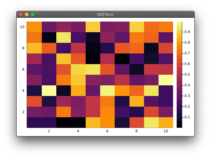

Git repository

Once you have your GitHub account ready (see lecture 2 how-to), create a private repository you will share with the teaching staff only to upload your weekly assignments (scripts):

1. Create a private GitHub repository named pde-on-gpu-<moodleprofilename>, where <moodleprofilename> has to be replaced by your name as displayed on Moodle, lowercase, diacritics removed, spacing replaced with hyphens (-). For example, if your Moodle profile name is "Joël Désirée van der Linde" your repository should be named pde-on-gpu-joel-desiree-van-der-linde.

2. Select an MIT License and add a README.md file.

3. Share this private repository on GitHub with the teaching-bot (https://github.com/teaching-bot).

4. For each homework submission, you will:

   • create a git branch named homework-X (X $\in [2-...]$) and switch to that branch (git switch -c homework-X);

   • create a new folder named homework-X to put the exercise codes into;

   • (don't forget to git add the code-files and git commit them);

   • push to GitHub and open a pull request (PR) on the main branch on GitHub;

   • copy the single git commit hash (or SHA) of the final push and the link to the PR and submit both on Moodle as the assignment hand-in (it will serve to control the material was pushed on time);

   • (do not merge the PR yet).

👉 See Logistics for details.

GitHub task

For this week:

First an edit without a PR

• edit the README.md of your private repository (add one or two description sentences in there (to get familiar with the Markdown syntax);

• commit this to the main branch (i.e. no PR) and push.

Second, an edit with a PR:

• create and switch to homework-2 branch;

• create a folder homework-2 and a file inside that folder homework-2/just-a-test with content This is to make a PR;

• push and create a PR.

Copy the commit hash (or SHA) and paste it to Moodle in the git commit hash (SHA) activity as well as the link to the PR.

⤴ back to Content